Working with 2.5D graphs
Now that we know what is an RNA 2.5D graph we can inspect the graph using rnaglib.
Fetching hosted graphs
The libray ships with some pre-built datasets which you can download with the following command line:
$ rnaglib_download
This will download the default data distribution to ~/.rnaglib
To see the list of available PDBs you downloaded, use:
from rnaglib.utils import available_pdbids
# returns a list of PDBIDs
pdbids = available_pdbids()
# get the first RNA by PDBID
rna = graph_from_pdbid(pdbids[0])
Warning
The list of available PDBs depends on which data build you want to use. See preparing data for more info on versioning and data build arguments. You can pass these arguments to the available_pdbids(redundancy=’all’, version=’0.0.0’, annotated=True) for non-default builds.
Overview of the 2.5D Graphs
First, let us have a look at the 2.5d graph object from a code perspective. We use networkx to store the RNA information in a nx.DiGraph directed graph object. Once the graphs are downloaded, they can be fetched directly using their PDBID.
Since nodes represent nucleotides, the node data dictionary will include features such as nucleotide type,
position, 3D coordinates, etc…
Nodes are assigned an ID in the form <pdbid.chain.position>.
Using node IDs we can access node and edge attributes as dictionary keys.
>>> from rnaglib.utils import graph_from_pdbid
>>> G = graph_from_pdbid("4nlf")
>>> G.nodes['4nlf.A.2647']
 {'index': 1, 'index_chain': 1, 'chain_name': 'A', 'nt_resnum': 2647, 'nt_name': 'U', 'nt_code': 'U',
  'binding_protein': None, 'binding_ion': None, 'binding_small-molecule': None}
The RNA 2.5D graph contains a rich set of annotations. For a complete list of these annotations see this page.
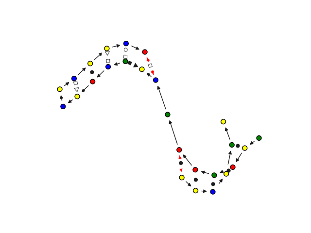
Visualization
To visualize the 2.5D graphs in the format described above, we have implemented a drawing toolbox with several
functions. The easiest way to use it in your application is to call rnaglib.drawing.draw(graph, show=True).
A functioning installation of Latex is needed for correct plotting of the graphs. If no installation is detected,
the graphs will be plotted using the LaTex reduced features that ships with matplotlib.
>>> from rnaglib.drawing import rna_draw
>>> rna_draw(G, show=True, layout="spring")
In the next two examples we will show how you can make use of these annotations to study chemical modifications and RNA-protein binding sites.
Analyzing RNA-small molecule binding sites
In this short example we will compute some statistics to describe the kinds of structural features around RNA-small molecule binding pockets using RNAGlib.
Let’s get our graphs. We are using the default data build which contains whole non-redundant RNA structures. We will iterate over all available non-redundant RNAs and extract residues near small molecules.
from rnaglib.utils import available_pdbids
from rnaglib.utils import graph_from_pdbid

pockets = []
for i,G in enumerate(graphs):
        try:
            pocket = [n for n, data in G.nodes(data=True) if data['binding_small-molecule'] is not None]
            # sample same number of random nucleotides
            non_pocket = random.sample(list(G.nodes()), k=len(pocket))
        except KeyError as e:
            continue
        if pocket:
            pockets.append((pocket, non_pocket, G))
        else:
            # no pocket found
            pass
Now we have a list of pockets where each is a thruple of a list of pocket nodes, a list of non-pocket nodes, and the parent graph. Let’s collect some stats about these residues. Namely, what base pair types and secondary structure elements they are involved in.
bps, sses = [], []

for pocket, non_pocket, G in pockets:
    for nt in pocket:
        # add edge type of all base pairs in pocket
        bps.extend([{'bp_type': data['LW'],
                     'is_pocket': True} for _,data in G[nt].items()])
        # sse key is format '<sse type>_<id>'
        node_data = G.nodes[nt]
        if node_data['sse']['sse'] is None:
            continue
        sses.append({'sse_type': node_data['sse']['sse'].split("_")[0],
                     'is_pocket': True})

    # do the same for non-pocket
    for nt in non_pocket:
        # add edge type of all base pairs in pocket
        bps.extend([{'bp_type': data['LW'],
                     'is_pocket': False} for _,data in G[nt].items()])
        # sse key is format '<sse type>_<id>'
        node_data = G.nodes[nt]
        if node_data['sse']['sse'] is None:
            continue
        sses.append({'sse_type': node_data['sse']['sse'].split("_")[0],
                     'is_pocket':False})


# for convenience convert to dataframe
bp_df = pd.DataFrame(bps)
sse_df = pd.DataFrame(sses)
Finally we can draw some plots of the base pair type and secondary structure element distribution around small molecule binding sites.
# remove backbones
bp_df = bp_df.loc[~bp_df['bp_type'].isin(['B35', 'B53'])]

sns.histplot(y='bp_type', hue='is_pocket', multiple='dodge', stat='proportion', data=bp_df)
sns.despine(left=True, bottom=True)
plt.savefig("bp.png")
plt.clf()

sns.histplot(y='sse_type', hue='is_pocket', multiple='dodge', stat='proportion', data=sse_df)
sns.despine(left=True, bottom=True)
plt.savefig("sse.png")
plt.clf()
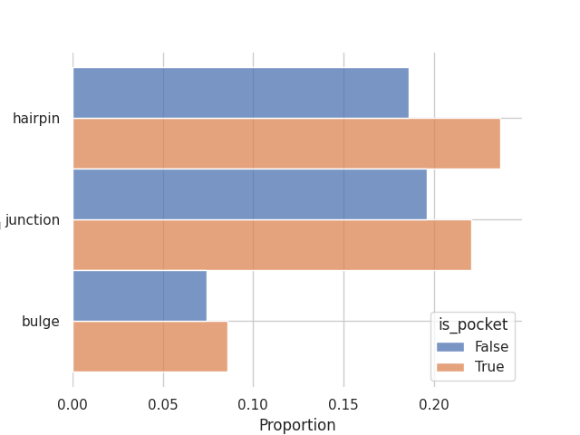
This is the distribution of secondary structures in binding pockets and in a random sample of residues:
And the same but for the different LW base pair geometries:
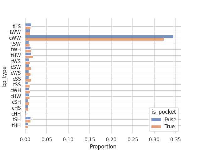
From this small experiment we confirm a property of RNA binding sites which is that they tend to occur in looping regions with a slight tendency towards non-canonical (non-CWW) base pair geometries.
Aligning two RNA graphs: Graph Edit Distance (GED)
GED is the gold standard of graph comparisons. We have put our ged implementation as a part of networkx, and offer
in rnaglib.ged the weighting scheme we propose to compare 2.5D graphs. One can call rnaglib.ged.ged() on two
graphs to compare them. However, due to the exponential complexity of the comparison, the maximum size of the graphs
should be around ten nodes, making it more suited for comparing graphlets or subgraphs.
>>> from rnaglib.ged import graph_edit_distance
>>> from rnaglib.utils import graph_from_pdbid
>>> G = graph_from_pdbid("4nlf")
>>> graph_edit_distance(G, G)
... 0.0
Using your own local RNA structures
If you have an mmCIF containing RNA stored locally and you wish to build a 2.5D graph that can be used in RNAglib you
can use the prepare_data module.
To do so, you need to have x3dna-dssr executable in your $PATH which requires a license <http://x3dna.org/>.
The first option is to use the library from a python script, following the example :
>>> from rnaglib.prepare_data import cif_to_graph

>>> pdb_path = '../data/1aju.cif'
>>> graph_nx = cif_to_graph(pdb_path)
Another possibility is to use the shell function that ships with rnaglib.
$ rnaglib_prepare_data --one_mmcif $PATH_TO_YOUR_MMCIF -O /path/to/output